Quickstart

In this quick example, we will calculate the lensing amplitude around galaxies in Baryon Oscillation Spectroscopic Survey (BOSS) in the redshift range \(0.2 < z_l < 0.4\) with the final release of the Kilo Degree Survey (KiDS). We start by downloading and processing the publicly available data. Note that the KiDS files alone are around 7 GB, so this may take a while.

from urllib.request import urlretrieve

from astropy.table import Table
from dsigma.scripts.process_kids_legacy import process_kids_legacy

# Download the BOSS data.
filename = "galaxy_DR12v5_CMASSLOWZTOT_North.fits.gz"
urlretrieve(f"https://data.sdss.org/sas/dr12/boss/lss/{filename}", filename)
table_l = Table.read(filename)
for key in ['Z', 'RA', 'DEC']:
    table_l.rename_column(key, key.lower())
table_l['w_sys'] = 1
table_l = table_l[(0.2 < table_l['z']) & (table_l['z'] < 0.4)]
table_l.keep_columns(['ra', 'dec', 'z', 'w_sys'])

# Download and process the KiDS data.
for filename in ["KiDS_Legacy_NS_unblind_final.fits.gz",
                 "KiDZ_Legacy_unblind_final.fits"]:
    urlretrieve(f"https://kids.strw.leidenuniv.nl/DR5/data_files/{filename}",
                filename)
process_kids_legacy()
table_s = Table.read('kids_legacy.hdf5', path='catalog')
table_n = Table.read('kids_legacy.hdf5', path='calibration')

The most computationally demanding step is the precomputation, where dsigma sums up contributions from lensed source galaxies around each lens. The result is stored directly in table_l. This is the most computationally demanding part of the process.

import numpy as np
from astropy import units as u
from astropy.cosmology import units as cu
from dsigma.precompute import precompute

rp_bins = np.logspace(-1, 1.4, 13) * u.Mpc / cu.littleh
precompute(table_l, table_s, rp_bins, table_n=table_n, progress_bar=True)

With the precomputation complete, we stack the signal across all lenses and use jackknife resampling to estimate uncertainties.

from dsigma.jackknife import compute_jackknife_fields, jackknife_resampling
from dsigma.stacking import excess_surface_density

compute_jackknife_fields(table_l, 100)
kwargs = dict(scalar_shear_response_correction=True)
results = excess_surface_density(table_l, return_table=True, **kwargs)
results['ds_err'] = np.sqrt(np.diag(jackknife_resampling(
    excess_surface_density, table_l, **kwargs)))

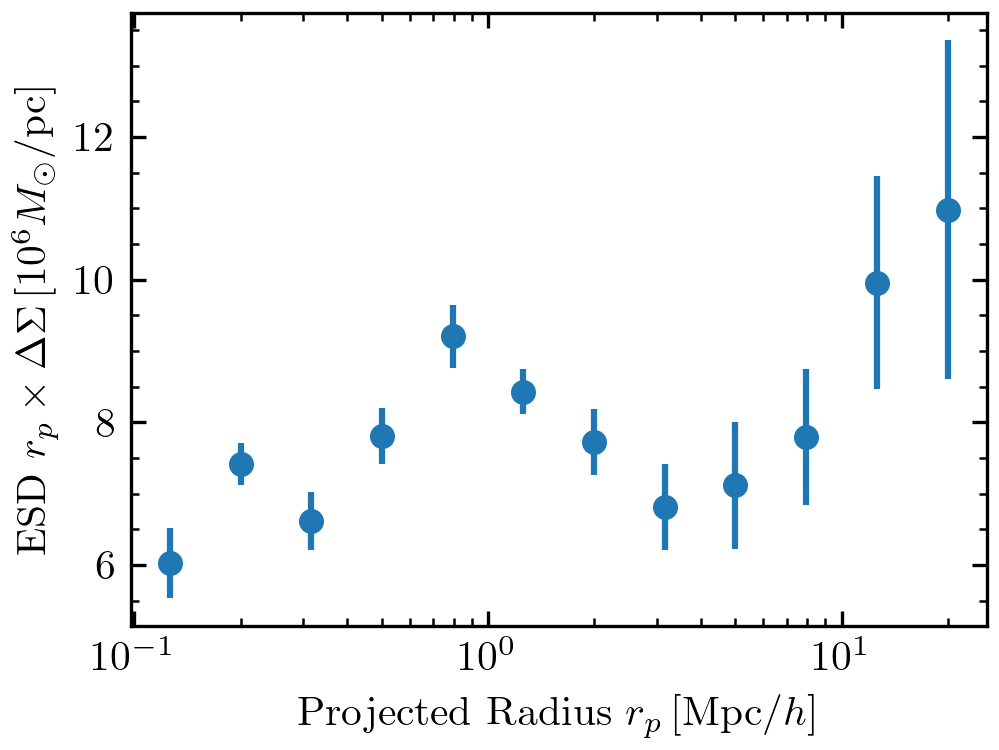
Finally, we plot the result using matplotlib.

import matplotlib.pyplot as plt

rp = np.sqrt(results['rp_min'] * results['rp_max'])
plt.errorbar(rp, rp * results['ds'], yerr=rp * results['ds_err'], fmt='o',
             ms=5)
plt.xscale('log')
plt.xlabel(r'Projected Radius $r_p \, [\mathrm{Mpc} / h]$')
plt.ylabel(r'ESD $r_p \times \Delta \Sigma \, [10^6 M_\odot / \mathrm{pc}]$')

For more details on each step, refer to the workflow and application pages.